Neural Networks for beginners
Building simple neural networks with Pytorch made easy!

Intro
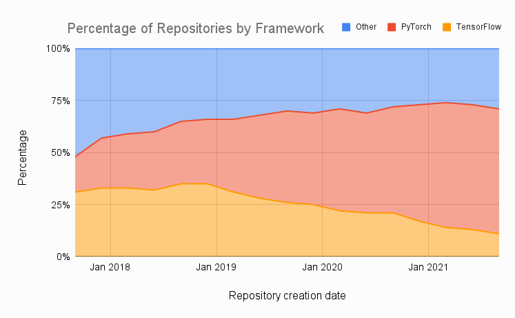
In this article, we will be creating a simple Neural Network using PyTorch and understanding the functions used. The reason for using PyTorch is that it has been used in research and model deployment purposes more than Tensorflow recently. For installation of PyTorch, you can refer to the official PyTorch website.
Starting with importing the PyTorch Library
import torch
import torch.nn as nn
import torch.optim as optim
import torch.nn.functional as F
from torch.utils.data import DataLoader
import torchvision.datasets as datasets
import torchvision.transforms as transforms
torch.nn provides us with all Neural Network Modules such as CNN, Rgivestorch.optim provides us with Optimizers such as SGD, Adam, etctorch.nn.functional provides us with Parameterless functions like activation functionstorch.utils.data helps with dataset management by creating mini-batches, etctorchvision.datasets helps to perform transformations on our dataset such as data augmentation
Creating Neural Network
Here we inherit the nn.Module which is a more general way to build Neural Networks and offers more flexibility. You can also use nn.Sequential for this example.
    def __init__(self,input_size,num_classes):
        super(NN,self).__init__()
        self.fc1 = nn.Linear(input_size,50)
        self.fc2 = nn.Linear(50,num_classes)
Here we create a fully connected Neural Network with 2 layers. We will be using the MNIST digit recognition dataset for training. Thus the input size for the first layer will be 784(28*28). The output of the first layer will be 50 which will be the input size for the second layer. The output of the second layer will be the number of classes (num_classes) which will be 10 (as in digits from 0-9).The function as no return values.
    def forward(self,x):
        x = F.relu(self.fc1(x))
        x = self.fc2(x)
        return x
In forward function above the 'x' is the MNIST images and we will run those images from fc1 and fc2 that we created in about __init__ function. In this function, we also use the ReLu activation function in between. The function returns x (MNIST images).
More about the ReLu activation function:
Activation functions are simple functions that transform inputs into outputs of a certain range. For example a sigmoid activation function takes inputs and maps the resulting value in between 0 to 1. One of the reasons activation functions are added in Neural Networks is that it helps the network to understand complex patterns in dataset.
ReLu stands for rectified linear activation and it maps the input in between 0 and x, i.e the function returns 0 if the value is negative and it returns the same input value if it is greater than 0.
Finally, our Neural Network class will look like this:
class NN(nn.Module):
    def __init__(self,input_size,num_classes):
        super(NN,self).__init__()
        self.fc1 = nn.Linear(input_size,50)
        self.fc2 = nn.Linear(50,num_classes)

    def forward(self,x):
        x = F.relu(self.fc1(x))
        x = self.fc2(x)
        return x
Deciding the Hyperparameters
Next, we set up the Hyperparameters for our Neural Network.
# Hyperparameters
input_size = 784
num_classes = 10
learning_rate = 0.001
batch_size = 64
num_epochs = 3
While training a Neural Network there are two kinds of parameters 1) Learnable Parameters and 2) Hyperparameters. Learnable parameters are parameters that the neural network learns on its own during training. Hyperparameters are the parameters that we provide to control the way algorithms learn.
Learning Rate
The learning rate is the hyperparameter that is used to control the rate at which the model updates its parameter estimates.
Batch size and Num epochs
Batch size is the number of samples processed before the model is updated. The number of epochs is the number of complete passes through the training dataset.
Loading data and Initializing Network
# Load Data
train_dataset = datasets.MNIST(root="dataset/", train=True, transform=transforms.ToTensor(), download=True)
test_dataset = datasets.MNIST(root="dataset/", train=False, transform=transforms.ToTensor(), download=True)
train_loader = DataLoader(dataset=train_dataset, batch_size=batch_size, shuffle=True)
test_loader = DataLoader(dataset=test_dataset, batch_size=batch_size, shuffle=True)

# Initialize network
model = NN(input_size=input_size, num_classes=num_classes)
Here we load the MNIST dataset and make use of transforms it to transform it into a tensor to train the network. DataLoader makes it easier for us to manage our dataset. We set shuffle=True to introduce randomness in our dataset while training. This might help us in avoiding overfitting. At last, we define our model.
Loss and Optimizer
# Loss and optimizer
criterion = nn.CrossEntropyLoss()
optimizer = optim.Adam(model.parameters(), lr=learning_rate)
When working on Deep learning models loss/cost functions are used to optimize the model during training. The objective is always to minimize the loss function. Lower the loss better the model. The cross-Entropy loss function is important. It is used to optimize classification models.
Adam is an adaptive learning rate optimization algorithm that’s been designed specifically for training deep neural networks. First published in 2014, Adam was presented at a very prestigious conference for deep learning practitioners. The paper contained some very promising diagrams, showing huge performance gains in terms of speed of training.
In this blog, we are not focusing on the mathematics of these functions. Our main focus here is to understand and implement the Pytorch library.
Training the Network
# Train Network
for epoch in range(num_epochs):
    for batch_idx, (data, targets) in enumerate(tqdm(train_loader)):
        # Get data to cuda if possible
        data = data.to(device=device)
        targets = targets.to(device=device)

        # Get to correct shape
        data = data.reshape(data.shape[0], -1)

        # Forward
        scores = model(data)
        loss = criterion(scores, targets)

        # Backward
        optimizer.zero_grad()
        loss.backward()

        # Gradient descent or adam step
        optimizer.step()
The above code is used to train the neural network. This code will be the same for Convolutional Neural Networks and Recurrent Neural Networks (only the data reshaping might change).
In PyTorch, for every mini-batch during the training phase, we typically want to explicitly set the gradients to zero before starting to do backpropagation (i.e., updating the Weights and biases) because PyTorch accumulates the gradients on subsequent backward passes. This accumulating behavior is convenient while training RNNs or when we want to compute the gradient of the loss summed over multiple mini-batches.
optimizer.step() is used to perform a single optimization step i.e to update the parameters.
Calculating Accuracy
# Check accuracy on training & test to see how good our model
def check_accuracy(loader, model):
num_correct = 0
num_samples = 0
model.eval()
with torch.no_grad():
# Loop through the data
for x, y in loader:
# Move data to device
x = x.to(device=device)
y = y.to(device=device)
# Get to correct shape
x = x.reshape(x.shape[0], -1)
97
# Forward pass
scores = model(x)
_, predictions = scores.max(1)
# Check how many we got correct
num_correct += (predictions == y).sum()
# Keep track of number of samples
num_samples += predictions.size(0)
model.train()
return num_correct/num_samples
# Check accuracy on training & test to see how good our model
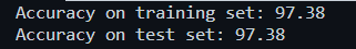
print(f"Accuracy on training set: {check_accuracy(train_loader, model)*100:.2f}")
print(f"Accuracy on test set: {check_accuracy(test_loader, model)*100:.2f}")
Just like the training of neural networks, the code for calculating accuracy will be the same for CNNs, RNNs, DNNs, etc (data reshaping might change).
Here we use torch.no_grad() because we don't need to keep track of gradients while calculating accuracy. tqdm is used for a nice progress bar!
Results
After training for 5 epochs only we get an accuracy of 97.38%.
Outro
Hope you understood each function we used to build a simple neural network. In the next blogs, we will see how to build CNNs, RNNs, and many more! The code for these will be similar.
If you like the content make sure to like and subscribe for more such articles.
